| .gitignore | ||
| image.ppm | ||
| LICENSE | ||
| main.go | ||
| README.md | ||
RaytracerGO
A raytracer and renderer writen in Go (Golang) following the book Raytracing in one weekend
Motivation
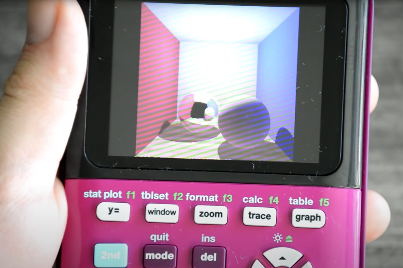
I've been meaning to tinker with graphics for quite a while and was motivated by a video programming a raytracing algorithm on a TI-84. Back in my school days I used to love to tinker with the TI-84 and also did some very elementary programming on it myself.
Video that started it all: Raytracing on a Graphing Calculator (again)
Why Go?
The story starts with Zig. A few colleagues of mine and I tried to work on a Guake-like browser using Zig. We chose Zig because it's C-like, modern and because their mascot is a lizard, of course. But I don't like Zig all that much, and right now Go has caught my attention.
I like the language a lot, it's still very C-like, doesn't have classes :), is open-source and resembles Python a lot, while still being fast and having crazy fast compiling speeds (which is something I've started to appreciate since dabbling with Linux From Scratch). The only draw back of Go is that it is a little bit slower than C++, but I just want to experience what the Python-version of C is like :)

Taglibro
Chapter 1: The PPM-image format
Yay this is the first image I've ever generated without using any external imported library ^^
Chapter 2: Vector operations: Ditching OOP for GO
Implemented the vec3 Class and colour utility functions without classes. Struktoj estas sufiĉa.
Chapter 3: Implementing the camera, rays and a background
To understand computer graphics better I will try to describe some important definitions with my own words:
- Rays: A ray is a 3D-vector with an origin pointing with some length in one direction (P(x)=O+x*b, where O is the origin and b is a vector pointing in one direction)
- Viewport: Is essentially a window (typically the user window) through which we see the 3D environment. Adjusting the viewport allows you to zoom in, pan around, or focus on specific areas of your scene.
- Camera: Is essentially a mathematical function (a virtual eye of sorts) that captures rays that originate from its position and pass through the viewport and generates an image that the user can see.
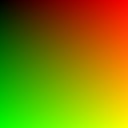
By the end of this chapter I generated the following background:

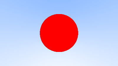
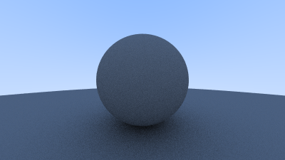
Chapter 4: Creating a sphere
In this chapter I created a simple sphere and detect its surface by solving quadratic equations, which represent vectors. The sphere has no shading yet:
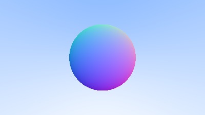
Chapter 5: Surface normals
The first part of the chapter was the calculation and visualization of the normals, which we need for shading. But I also implemented the fast inverse square algorithm in Go just like in Quake III, which is pretty clever and fast. I did primarily because 1) I'm working with 32-bit floats for the sake of memory efficiency and 2) I don't care about accuracy - also it's very educational. But as explained in this video the fast inverse square isn't always the better choice and in my case it probably isn't, because I need to import a Go standard library to disable data type safety and processor padding (something I've noticed when working with small data types in Zig). This is the first visualization of the normals of the sphere:
The second part of the capter involved standardizing the code so that it can process multiple objects - it was quite translating this part into Go, as a lot of C++ OOP features are missing - but finally I managed to produce this neat output:
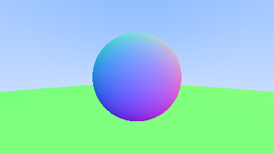
At the end I also added an intervals struct, to further simplify the code.
Chapter 6: The Camera struct
This chapter was yet another simplification of the existing code - the viewport and the camera were moved out of main and got their own struct. The camera struct and the render function have two tasks:
- Construct and dispatch rays into the world and
- Use the results of these rays to construct the rendered image
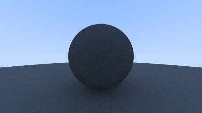
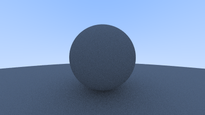
Chapter 7: Anti-Aliasing
The images rendered thus far have jagged edges and this is known as aliasing. To soften the edges each pixel gets sampled multiple times and the colour gets averaged. I've spend quite some time on this chapter due to a veeeery small bug in the code. This chapter produces a similar but softer image as before. Here an comparison:

This is also the first time the code starts to take some time to execute.
Chapter 8: Diffuse objects
A diffuse object is any object that is not emitting light, takes on the colours of the environment and reflects light in all directions.

I generated random reflection vectors and got the following (this is the first time a shadow can be observed, left one is mine, right one from the book - note the stripe is probably a consequence of fast inverse square and of using 32-bit floats instead of 64-bit ones):

A problem that occurs on this image is the shadow acne problem: A ray will attempt to accurately calculate the intersection point when it intersects with a surface. Unfortunately for us, this calculation is susceptible to floating point rounding errors which can cause the intersection point to be ever so slightly off. This means that the origin of the next ray, the ray that is randomly scattered off of the surface, is unlikely to be perfectly flush with the surface. It might be just above the surface. It might be just below the surface. If the ray's origin is just below the surface then it could intersect with that surface again. Which means that it will find the nearest surface at t=0.00000001 or whatever floating point approximation the hit function gives us. The simple fix yields this image:
To make the shadows look more realistic, I had to implement the Lambertian reflections: basically, most of the reflected rays will be close to the sphere normal and the probability density is dependent on cos(phi), where phi is the angle from the normal. It was very easy to implement and yields the following:
The last issue left in the chapter is the darkness of the image and it's due to some strange linear-gamma space conversion? I don't quite understand how that works, but by taking the square root of the colour values we get the right brightness. Nice

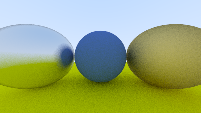
Chapter 8: The Materials struct and Metals
In this chapter I made a special struct that saves the properties of the material (its fuzz and albedo) and checks whether it is lambertian or metallic. Working without OOP gets a bit awkward here and I had some problems with debugging (due to pointers). But reflections on metals really do look nice:
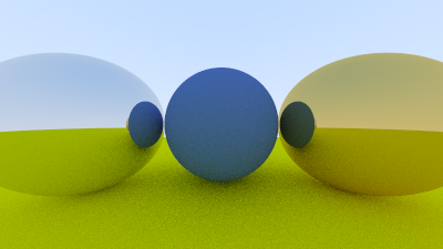
Most metals however aren't purely reflective, they fuzz the reflection a little bit - so they are actually something inbetween a lambertian object and a mirror. Accounting for this gives the following neat image: